Getting Started

System Requirements

MC3 (version 1.2) is known to work on Unix/Linux (Ubuntu) and OSX (10.9+) machines, with the following software:

• Python (version 2.7)
• Numpy (version 1.8.2+)
• Scipy (version 0.13.3+)
• Matplotlib (version 1.3.1+)
• mpi4py (version 1.3.1+)
• Message Passing Interface, MPI (MPICH preferred)

MC3 may work with previous versions of these software; however, we do not guarantee nor provide support for that.

Install

To obtain the latest MCcubed code, clone the repository to your local machine with the following terminal commands. First, keep track of the folder where you are putting MC3:

topdir=`pwd`
git clone https://github.com/pcubillos/MCcubed

Compile

Compile the C-extensions of the package:

cd $topdir/MCcubed/
make

To remove the program binaries, execute (from the respective directories):

make clean

Example 1 (Interactive)

The following example (demo01) shows a basic MCMC run with MC3 from the Python interpreter. This example fits a quadratic polynomial curve to a dataset. First create a folder to run the example (alternatively, run the example from any location, but adjust the paths of the Python script):

cd $topdir
mkdir run01
cd run01

Now start a Python interactive session. This script imports the necesary modules, creates a noisy dataset, and runs the MCMC:

import sys
import numpy as np
import matplotlib.pyplot as plt
sys.path.append("../MCcubed/")
import MCcubed as mc3

# Get function to model (and sample):
sys.path.append("../MCcubed/examples/models/")
from quadratic import quad

# Create a synthetic dataset:
x = np.linspace(0, 10, 100)          # Independent model variable
p0 = 3, -2.4, 0.5                    # True-underlying model parameters
y = quad(p0, x)                      # Noiseless model
uncert = np.sqrt(np.abs(y))          # Data points uncertainty
error = np.random.normal(0, uncert)  # Noise for the data
data = y + error                     # Noisy data set

# Fit the quad polynomial coefficients:
params = np.array([ 20.0, -2.0, 0.1])  # Initial guess of fitting params.

# Run the MCMC:
posterior, bestp = mc3.mcmc(data, uncert, func=quad, indparams=[x],
                            params=params, numit=3e4, burnin=100)

Outputs

That’s it, now let’s see the results. MC3 will print out to screen a progress report every 10% of the MCMC run, showing the time, number of times a parameter tried to go beyond the boundaries, the current best-fitting values, and corresponding \(\chi^{2}\); for example:

::::::::::::::::::::::::::::::::::::::::::::::::::::::::::::::::::::::
  Multi-Core Markov-Chain Monte Carlo (MC3).
  Version 1.2.0.
  Copyright (c) 2015-2016 Patricio Cubillos and collaborators.
  MC3 is open-source software under the MIT license (see LICENSE).
::::::::::::::::::::::::::::::::::::::::::::::::::::::::::::::::::::::

Start MCMC chains  (Fri Feb  5 10:45:17 2016)

[:         ]  10.0% completed  (Fri Feb  5 10:45:17 2016)
Out-of-bound Trials:
 [0 0 0]
Best Parameters:   (chisq=111.0541)
[ 3.79473869 -2.73050517  0.51636233]

...

[::::::::::] 100.0% completed  (Fri Feb  5 10:45:18 2016)
Out-of-bound Trials:
 [0 0 0]
Best Parameters:   (chisq=111.0449)
[ 3.77284276 -2.72330815  0.51634107]

Fin, MCMC Summary:
------------------
 Burned in iterations per chain:   100
 Number of iterations per chain:  3000
 MCMC sample size:               29000
 Acceptance rate:   39.04%

 Best-fit params   Uncertainties        S/N      Sample Mean   Note
   3.7728428e+00   3.8407332e-01       9.82    3.7694995e+00
  -2.7233081e+00   2.1964109e-01      12.40   -2.7232216e+00
   5.1634107e-01   2.6891868e-02      19.20    5.1641806e-01

 Best-parameter's chi-squared:     111.0449
 Bayesian Information Criterion:   124.8604
 Reduced chi-squared:                1.1448
 Standard deviation of residuals:  2.93518

At the end of the MCMC run, MC3 displays a summary of the MCMC sample, best-fitting parameters, uncertainties, mean values, and other statistics.

Note

More information will be displayed, depending on the MCMC configuration (see the Tutorial).

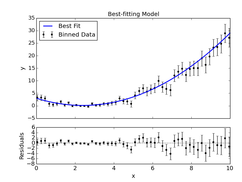
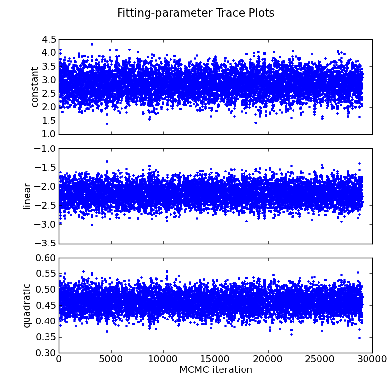
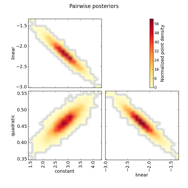
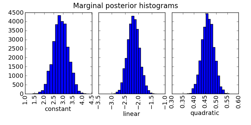
Additionally, the user has the option to generate several plots of the MCMC sample: the best-fitting model and data curves, parameter traces, and marginal and pair-wise posteriors (these plots can also be generated automatically with the MCMC run). The plots sub-package provides the plotting functions:

# Plot best-fitting model and binned data:
mc3.plots.modelfit(data, uncert, x, y, title="Best-fitting Model",
                   savefile="quad_bestfit.png")
# Plot trace plot:
parname = ["constant", "linear", "quadratic"]
mc3.plots.trace(posterior, title="Fitting-parameter Trace Plots",
                parname=parname, savefile="quad_trace.png")

# Plot pairwise posteriors:
mc3.plots.pairwise(posterior, title="Pairwise posteriors", parname=parname,
                   savefile="quad_pairwise.png")

# Plot marginal posterior histograms:
mc3.plots.histogram(posterior, title="Marginal posterior histograms",
                    parname=parname, savefile="quad_hist.png")

Note

These plots can also be automatically generated along with the MCMC run (see File Outputs).

Example 2 (Shell Run)

The following example (demo02) shows a basic MCMC run from the shell prompt. To start, create a working directory to place the files and execute the program:

cd $topdir
mkdir run02
cd run02

Copy the demo files to run MC3 (configuration and data files):

cp $topdir/MCcubed/examples/demo02/* .

Call the MC3 executable, providing the configuration file as command-line argument:

mpirun $topdir/MCcubed/MCcubed/mccubed.py -c MCMC.cfg

Note

If you don’t have MPI or dont want to use it, make the previous call as:

python $topdir/MCcubed/MCcubed/mccubed.py -c MCMC.cfg

Noting that, in this last case, you need to have mpi=False.