Time Averaging
The MCcubed.rednoise.binrms routine computes the binned RMS array
(as function of bin size) used in the the time-averaging procedure.
Given a (model-data) residuals array. The routine returns the RMS of
the binend data (\({\rm rms}_N\)), the lower and upper RMS
uncertainties, the extrapolated RMS for Gaussian (white) noise
(\(\sigma_N\)), and the bin-size array (\(N\)).
This function uses an asymptotic approximation to compute the RMS uncertainties (\(\sigma_{\rm rms} = \sqrt{{\rm rms}_N / 2M}\)) for number of bins \(M> 35\). For smaller values of \(M\) (equivalently, large bin size) this routine computes the errors from the posterior PDF of the RMS (an inverse-gamma distribution). See [Cubillos2017].
Example
import numpy as np
import matplotlib.pyplot as plt
import MCcubed as mc3 # Add path to mc3 if necessary
plt.ion()
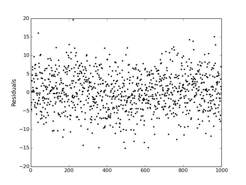
# Generate residuals signal:
N = 1000
# White-noise signal:
white = np.random.normal(0, 5, N)
# (Sinusoidal) time-correlated signal:
red = np.sin(np.arange(N)/(0.1*N))*np.random.normal(1.0, 1.0, N)
# Plot the time-correlated residuals signal:
plt.figure(0)
plt.clf()
plt.plot(white+red, ".k")
plt.ylabel("Residuals", fontsize=14)
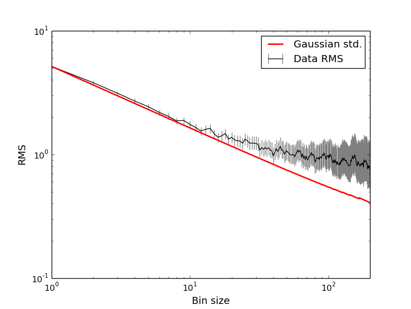
# Compute the residuals rms-vs-binsize:
maxbins = N/5
rms, rmslo, rmshi, stderr, binsz = mc3.rednoise.binrms(white+red, maxbins)
# Plot the rms with error bars along with the Gaussian standard deviation curve:
plt.figure(-6)
plt.clf()
plt.errorbar(binsz, rms, yerr=[rmslo, rmshi], fmt="k-", ecolor='0.5', capsize=0, label="Data RMS")
plt.loglog(binsz, stderr, color='red', ls='-', lw=2, label="Gaussian std.")
plt.xlim(1,200)
plt.legend(loc="upper right")
plt.xlabel("Bin size", fontsize=14)
plt.ylabel("RMS", fontsize=14)