Optimization Tutorial¶

This tutorial describes mc3’s optimization function mc3.fit(), which provides model-fitting optimization through scipy.optimize’s leastsq (Levenberg-Marquardt) and least_squares (Trust Region Reflective) routines. Additionally, the optimization can include (two-sided) Gaussian priors, set shared parameters, and fixed parameters. The mc3.fit() arguments work similarly to those of the mc3.sample() function.

This function performs a Maximum-A-Posteriori optimization by maximizing log_post (where we are neglecting the constant terms):

\[\begin{split}{\rm log\_post} &\equiv& \log({\rm likelihood}) + \log({\rm prior}), \\ &=& -\chi^2/2 + \log({\rm prior}), \\\end{split}\]

where the first term is the well known chi-square:

\[\chi^2 = \sum_i \left(\frac{{\rm data}_i - {\rm model}_i}{{\rm uncert}_i}\right)^2.\]

For the prior, the code computes log_prior as (once again neglecting constant terms):

\[{\rm log\_prior} \equiv \log({\rm prior}) = -\frac{1}{2} \sum_j \left(\frac{{\rm prior}_j - {\rm params}_j}{{\rm prior\_uncert}_j}\right)^2,\]

for each parameter with a Gaussian prior \(j\); parameters with uniform priors do not contribute to log_prior.

Basic Fit¶

This is the function’s calling signature:

mc3.fit(data, uncert, func, params, indparams=[], indparams_dict={}, pstep=None, pmin=None, pmax=None, prior=None, priorlow=None, priorup=None, leastsq='lm')[source]

In the most basic form, the user only needs to provide the fitting parameters and function, the data and \(1\sigma\)-uncertainties arrays, (and any additional argument to the fitting function). This will perform a Levenberg-Marquardt fit. The function returns a dictionary containing the best-fitting parameters, chi-square, and model, and the output from the scipy optimizer. See the example below:

import numpy as np
import mc3

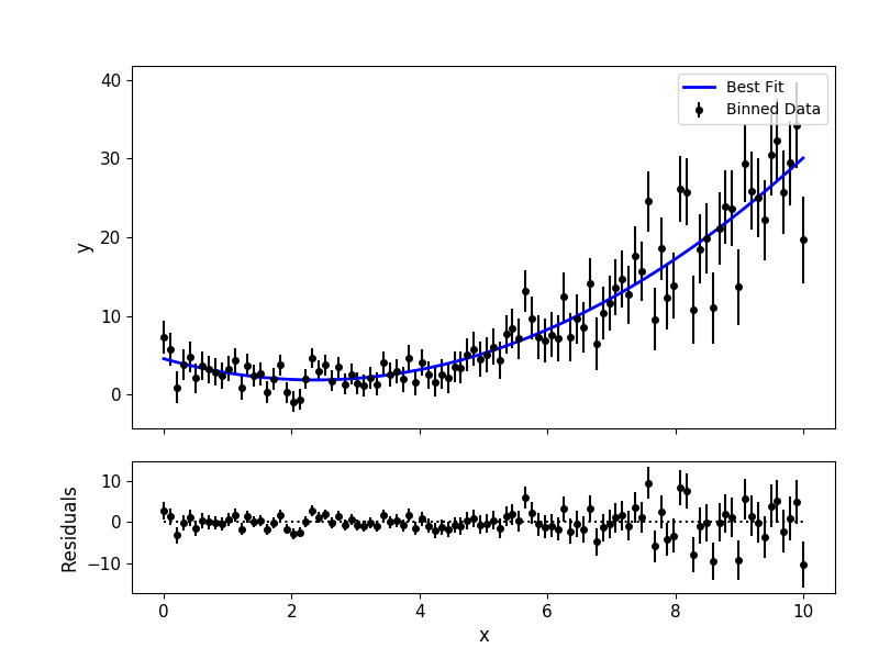
def quad(p, x):
    """Quadratic polynomial: y(x) = p0 + p1*x + p2*x^2"""
    return p[0] + p[1]*x + p[2]*x**2.0

# Preamble (create a synthetic dataset, in a real scenario you would
# get your dataset from your own data analysis pipeline):
np.random.seed(10)
x  = np.linspace(0, 10, 100)
p0 = [4.5, -2.4, 0.5]
y  = quad(p0, x)
uncert = np.sqrt(np.abs(y))
data   = y + np.random.normal(0, uncert)

# Fit the data:
output = mc3.fit(data, uncert, quad, [3.0, -2.0, 0.1], indparams=[x])

print(list(output.keys()))
['bestp', 'best_log_post', 'best_chisq', 'best_model', 'optimizer_res']

print(output['bestp'])
[ 4.57471072 -2.28357843  0.48341911]

# -2*log_post and chi-square are the same (uniform priors):
print(-2*output['best_log_post'], output['best_chisq'], sep='\n')
92.79923183159411
92.79923183159411

# Plot data and best-fitting model:
mc3.plots.modelfit(data, uncert, x, output['best_model'], nbins=100)

Data and Uncertainties¶

The data and uncert arguments are 1D arrays that set the data and \(1\sigma\) uncertainties to be fit.

Modeling Function¶

The func argument is a callable that defines the parameterized modeling function fitting the data. The only requirement for the modeling function is that its arguments follow the same structure of the callable in scipy.optimize.leastsq, i.e., the modeling function has to able to be called as: model = func(params, *indparams, **indparams_dict)

The params argument is a 1D array containing the initial-guess values for the model fitting parameters.

The indparams and indparams_dict arguments (optional) set any func additional argument as a list or keyword dictionary, respectively.

Optimization Algorithm¶

Set leastsq='lm' to use the Levenberg-Marquardt algorithm (default) via Scipy’s leastsq, or set leastsq='trf' to use the Trust Region Reflective algorithm via Scipy’s least_squares. Fixed and shared-values apply during the optimization (see Stepping Behavior), as well as the priors (see Parameter Priors).

Note

From the scipy documentation: Levenberg-Marquardt ‘doesn’t handle bounds’ but is ‘the most efficient method for small unconstrained problems’; whereas the Trust Region Reflective algorithm is a ‘Generally robust method, suitable for large sparse problems with bounds’.

The pmin and pmax arguments set the parameter lower and upper boundaries for a trf optimization, e.g:

# Fit with the 'trf' algorithm and bounded parameter space:
output = mc3.fit(data, uncert, quad, [4.5, -2.5, 0.5], indparams=[x],
    pmin=[4.4, -3.0, 0.4], pmax=[5.0, -2.0, 0.6], leastsq='trf')

Parameter Priors¶

The prior, priorlow, and priorup arguments (optional) set the prior probability distributions of the fitting parameters. Each of these arguments is a 1D float ndarray.

A priorlow value of zero (default) sets a uniform prior. This is appropriate when there is no prior knowledge of the value of a parameter \(\theta\):

\[p(\theta) = \frac{1}{\theta_{\rm max} - \theta_{\rm min}},\]

Positive values of priorlow and priorup set a Gaussian prior. This is typically used when a parameters has a previous estimate in the form of \(p(\theta) = {\theta_p\,}^{+\sigma_{\rm up}}_{-\sigma_\rm{lo}}\), where the values of prior, priorlow and priorup define the prior value, lower, and upper \(1\sigma\) uncertainties, respectively:

\[p(\theta) = A \exp\left(\frac{-(\theta-\theta_{p})^{2}}{2\sigma_{p}^{2}}\right),\]

where \(\sigma_{p}\) adopts the value of \(\sigma_{\rm lo}\) if \(\theta < \theta_p\), or \(\sigma_{\rm up}\) otherwise. The leading factor is given by \(A = 2/(\sqrt{2\pi}(\sigma_{\rm up}+\sigma_{\rm lo}))\) (see [Wallis2014]).

# (Following on the script above)
# Fit, imposing a Gaussian prior on the first parameter at 4.5 +/- 0.1,
# and leaving uniform priors for the rest:
prior    = np.array([ 4.0,  0.0,   0.0])
priorlow = np.array([ 0.1,  0.0,   0.0])
priorup  = np.array([ 0.1,  0.0,   0.0])
output = mc3.fit(data, uncert, quad, [3.0, -2.0,  0.1], indparams=[x],
    prior=prior, priorlow=priorlow, priorup=priorup)

# Best-fit solution is dominated by the prior on the first parameter:
print(output['bestp'])
[ 4.01743461 -2.00989432  0.45686521]

# -2*log_post and chi-square now differ:
print(-2*output['best_log_post'], output['best_chisq'], sep='\n')
93.8012177730325
93.7708211946111