Getting Started
System Requirements
mc3 is compatible with Python 3.9+, and has been tested to work on Unix/Linux and OS X machines.
Install
To install mc3 run the following command from the terminal:
pip install mc3
Or if you prefer conda:
conda install -c conda-forge mc3
Alternatively (e.g., for developers), clone the repository to your local machine with the following terminal commands:
git clone https://github.com/pcubillos/mc3
cd mc3
pip install -r requirements.txt
pip install -e .
mc3 provides MCMC posterior sampling,
optimization and other lower-level statistical and plotting
routines. See the full docs in the api or through the Python
interpreter:
import mc3
# Bayesian posterior sampling:
help(mc3.sample)

# Optimization:
help(mc3.fit)

# Assorted stats utilities:
help(mc3.stats)

# Plotting utilities:
help(mc3.plots)
Example 1: Interactive Run
The following example shows a basic MCMC run from the Python interpreter, for a quadratic-polynomial fit to a noisy dataset:
import numpy as np
import mc3


def quad(p, x):
    """
    Quadratic polynomial function.

    Parameters
        p: Polynomial constant, linear, and quadratic coefficients.
        x: Array of dependent variables where to evaluate the polynomial.
    Returns
        y: Polinomial evaluated at x:  y = p0 + p1*x + p2*x^2
    """
    y = p[0] + p[1]*x + p[2]*x**2.0
    return y

# For the sake of example, create a noisy synthetic dataset, in a real
# scenario you would get your dataset from your data analysis pipeline:
np.random.seed(3)
x = np.linspace(0, 10, 100)
p_true = [3.0, -2.4, 0.5]
y = quad(p_true, x)
uncert = np.sqrt(np.abs(y))
data = y + np.random.normal(0, uncert)

# Initial guess for fitting parameters:
params = np.array([10.0, -2.0, 0.1])
pstep  = np.array([0.03, 0.03, 0.05])

# Run the MCMC:
func = quad
output = mc3.sample(
    data, uncert, func, params, indparams=[x],
    pstep=pstep, sampler='snooker', nsamples=1e5, burnin=1000, ncpu=7,
)
That’s it. The code returns a dictionary with the MCMC results.
Among these, you can find the posterior sample
(posterior), the best-fitting values (bestp),
the lower and upper boundaries of the 68%-credible region (CRlo
and CRhi, with respect to bestp), the standard deviation of
the marginal posteriors (stdp), among other variables.
mc3 will also print out to screen a progress report every 10% of
the MCMC run, showing the time, number of times a parameter tried to
go beyond the boundaries, the current best-fitting values, and
lowest \(\chi^{2}\); for example:
::::::::::::::::::::::::::::::::::::::::::::::::::::::::::::::::::::::
  Multi-core Markov-chain Monte Carlo (mc3).
  Version 3.1.0.
  Copyright (c) 2015-2023 Patricio Cubillos and collaborators.
  mc3 is open-source software under the MIT license (see LICENSE).
::::::::::::::::::::::::::::::::::::::::::::::::::::::::::::::::::::::

Yippee Ki Yay Monte Carlo!
Start MCMC chains  (Wed Mar 29 17:52:45 2023)

[:         ]  10.0% completed  (Wed Mar 29 17:52:46 2023)
Out-of-bound Trials:
[0 0 0]
Best Parameters: (chisq=112.6196)
[ 3.12005211 -2.51498098  0.50946457]
Gelman-Rubin statistics for free parameters:
[1.05031159 1.04920662 1.05254562]

...

[::::::::::] 100.0% completed  (Wed Mar 29 17:52:51 2023)
Out-of-bound Trials:
[0 0 0]
Best Parameters: (chisq=112.5923)
[ 3.07675149 -2.50001621  0.50890678]
Gelman-Rubin statistics for free parameters:
[1.00024775 1.00029444 1.00023952]
All parameters converged to within 1% of unity.

MCMC Summary:
-------------
  Number of evaluated samples:        100002
  Number of parallel chains:               7
  Average iterations per chain:        14286
  Burned-in iterations per chain:       1000
  Thinning factor:                         1
  MCMC sample size (thinned, burned):  93002
  Acceptance rate:   28.36%

Parameter name     best fit   median      1sigma_low   1sigma_hi        S/N
--------------- -----------  -----------------------------------  ---------
Param 1          3.0768e+00   3.0761e+00 -3.7968e-01  3.8946e-01        7.9
Param 2         -2.5000e+00  -2.4981e+00 -2.2876e-01  2.1325e-01       11.2
Param 3          5.0891e-01   5.0868e-01 -2.6467e-02  2.7415e-02       18.7

  Best-parameter's chi-squared:       112.5923
  Best-parameter's -2*log(posterior): 112.5923
  Bayesian Information Criterion:     126.4078
  Reduced chi-squared:                  1.1607
  Standard deviation of residuals:  3.00577

For a detailed summary with all parameter posterior statistics see
mc3_statistics.txt

Output sampler files:
  mc3_statistics.txt
At the end of the MCMC run, mc3 displays a summary of the MCMC
sample, best-fitting parameters, credible-region boundaries, posterior
mean and standard deviation, among other statistics.
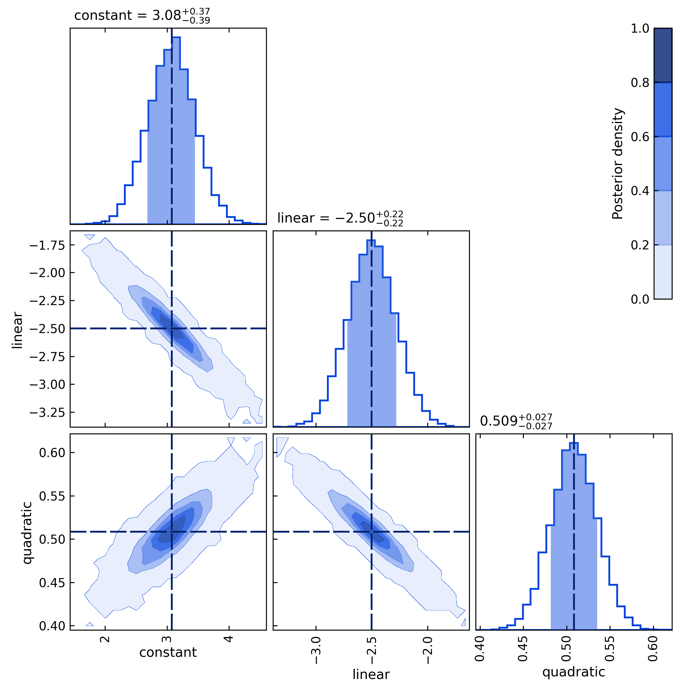
Additionally, the user has the option to generate several plots of the MCMC
sample: the best-fitting model and data curves, parameter traces, and
marginal and pair-wise posteriors (these plots can also be generated
automatically with the MCMC run by setting plots=True).
The plots sub-package provides the plotting functions:
# And now, some post processing:
import mc3.plots as mp
import mc3.utils as mu
# Output dict contains the entire sample (posterior), need to remove burn-in:
posterior, zchain, zmask = mu.burn(output)
# Set parameter names:
pnames = ["constant", "linear", "quadratic"]
post = mp.Posterior(posterior, pnames)
# Plot pairwise posteriors:
fig_pairs = post.plot(savefile="quad_pairwise.png")
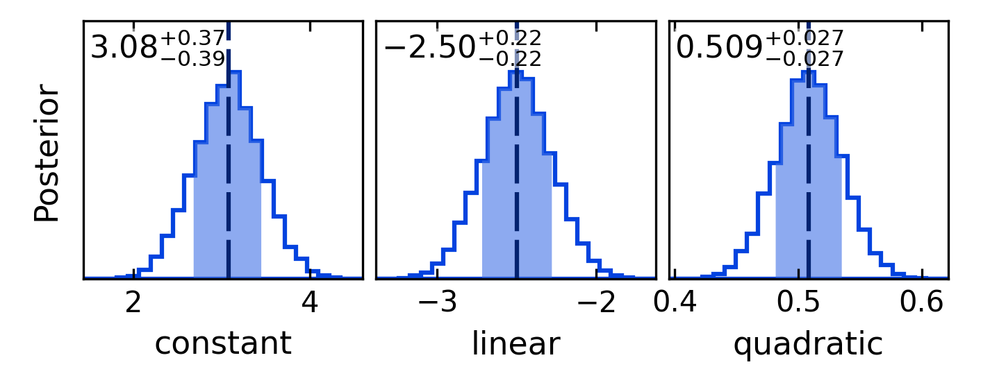
# Plot marginal posterior histograms:
fig_hist = post.plot_histogram(savefile="quad_hist.png")
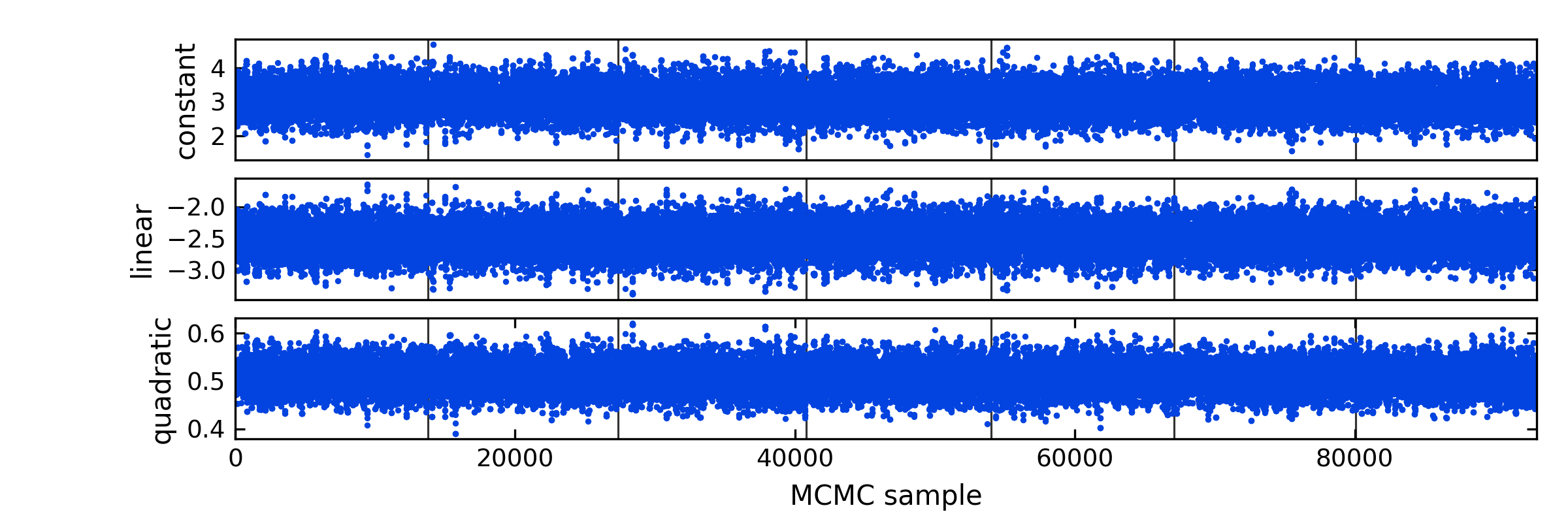
# Plot trace plot:
mp.trace(posterior, zchain, pnames=pnames, savefile="quad_trace.png")
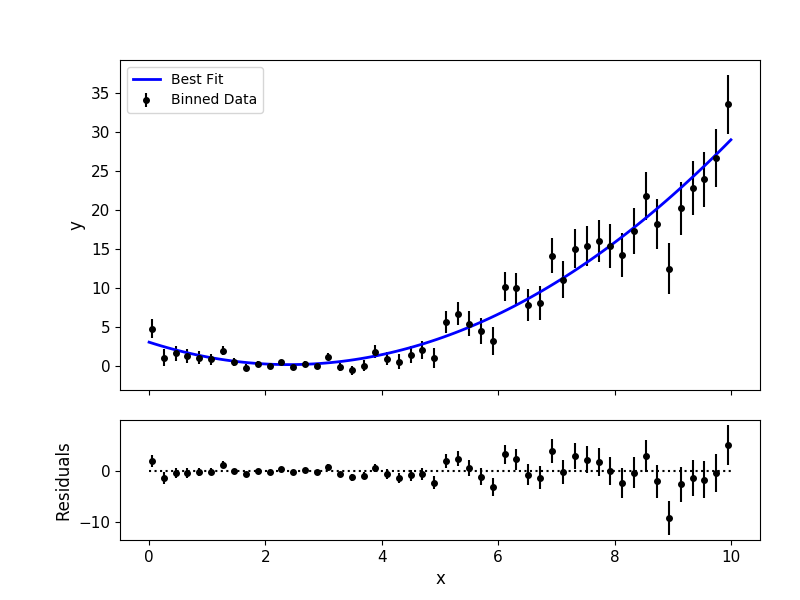
# Plot best-fitting model and binned data:
mp.modelfit(data, uncert, x, y, savefile="quad_bestfit.png")
Note
These plots can also be automatically generated along with the MCMC run (see Outputs).
Example 2: Shell Run
The following example shows a basic MCMC run from the terminal using a configuration file. First, create a Python file (’quadratic.py’) with the modeling function:
def quad(p, x):
    y = p[0] + p[1]*x + p[2]*x**2.0
    return y
Then, generate a data set and store into files, e.g., with the following Python script:
import numpy as np
import mc3
from quadratic import quad

# Create synthetic dataset:
x  = np.linspace(0, 10, 1000)         # Independent model variable
p0 = [3, -2.4, 0.5]                   # True-underlying model parameters
y  = quad(p0, x)                      # Noiseless model
uncert = np.sqrt(np.abs(y))           # Data points uncertainty
error = np.random.normal(0, uncert)   # Noise for the data
data = y + error                      # Noisy data set
# Store data set and other inputs:
mc3.utils.savebin([data, uncert], 'data.npz')
mc3.utils.savebin([x], 'indp.npz')
Now, create a configuration file with the mc3 setup (’MCMC.cfg’):
[MCMC]
data      = data.npz
indparams = indp.npz

func     = quad quadratic
params   =  10.0   -2.0   0.1
pmin     = -25.0  -10.0 -10.0
pmax     =  30.0   10.0  10.0
pstep    =   0.3    0.3   0.05

nsamples = 1e5
burnin   = 1000
ncpu     = 7
sampler  = snooker
grtest   = True
plots    = True
savefile = output_demo.npz
Finally, call the mc3 entry point, providing the configuration file as
a command-line argument:
mc3 -c MCMC.cfg