Time Averaging

The mc3.stats.time_avg() routine computes the binned RMS array (as function of bin size) used in the the time-averaging procedure for a given model–data residuals array. The routine returns the RMS of the binned data (\({\rm rms}_N\)), the lower and upper RMS uncertainties, the extrapolated RMS for Gaussian (white) noise (\(\sigma_N\)), and the bin-size array (\(N\)).

This function uses an asymptotic approximation to compute the RMS uncertainties (\(\sigma_{\rm rms} = \sqrt{{\rm rms}_N / 2M}\)) for number of bins \(M> 35\). For smaller values of \(M\) (equivalently, large bin size) this routine computes the errors from the posterior PDF of the RMS (an inverse-gamma distribution). For more details, see [Cubillos2017].

Example

For the sake of illustration, this example uses mock data. In the real world, your ‘data’ should be the residuals between the observed values and some model fit:

import numpy as np
import matplotlib.pyplot as plt
plt.ion()
import mc3.stats as ms


# Generate mock residuals signals:
N = 1000
np.random.seed(16)
# White-noise signal:
white = np.random.normal(0, 5, N)
# (Sinusoidal) time-correlated signal:
red = np.sin(np.arange(N)/(0.1*N))*np.random.normal(1.0, 1.0, N)

# Plot the time-correlated residuals signal:
plt.figure(0)
plt.clf()
plt.plot(white+red, ".k")
plt.ylabel("Residuals", fontsize=14)

# Compute the residuals rms-vs-binsize for a non-correlated and a time-correlated signal:
maxbins = N//5
white_rms, white_rmslo, white_rmshi, white_stderr, binsz = ms.time_avg(white,     maxbins)
red_rms,   red_rmslo,   red_rmshi,   red_stderr,   binsz = ms.time_avg(white+red, maxbins)

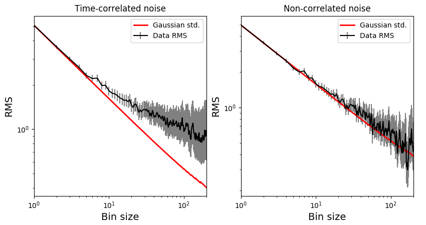
# Plot the rms with error bars along with the Gaussian standard deviation curve:
plt.figure(16)
plt.clf()
plt.title('Time-correlated noise')
plt.errorbar(binsz, red_rms, yerr=[red_rmslo, red_rmshi], fmt="k-",
    ecolor='0.5', capsize=0, label="Data RMS")
plt.loglog(binsz, red_stderr, color='red', ls='-', lw=2, label="Gaussian std.")
plt.xlim(1,200)
plt.legend(loc="upper right")
plt.xlabel("Bin size", fontsize=14)
plt.ylabel("RMS", fontsize=14)

plt.figure(17)
plt.clf()
plt.title('Non-correlated noise')
plt.errorbar(binsz, white_rms, yerr=[white_rmslo, white_rmshi], fmt="k-",
    ecolor='0.5', capsize=0, label="Data RMS")
plt.loglog(binsz, white_stderr, color='red', ls='-', lw=2, label="Gaussian std.")
plt.xlim(1,200)
plt.legend(loc="upper right")
plt.xlabel("Bin size", fontsize=14)
plt.ylabel("RMS", fontsize=14)

For a time-correlated signal, the RMS-vs-binsize curve deviates above the white-noise Gaussian prediction, as in the left panel below. For a white-noise signal, both curves should match within uncertainties, as in the right panel below: